My best Excel PivotTables start with these 4 functions

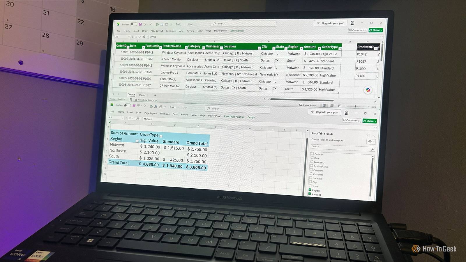
Published Aug 23, 2026, 3:30 PM EDT Tony Phillips is an experienced Microsoft Office user with a dual-honors degree in Linguistics and Hispanic Studies. Prior to starting with How-to Geek in January 2024, he worked as a document producer, data manager, and content creator for over ten years, and loves making spreadsheets and documents in his spare time. Tony is also an academic proofreader, experienced in reading, editing, and formatting over 3 million words of personal statements, resumes, reference letters, research proposals, and dissertations. Before joining How-To Geek, Tony formatted and wrote documents for legal firms, including contracts, Wills, and Powers of Attorney. Tony is obsessed with Microsoft Office! He will find any reason to create a spreadsheet, exploring ways to add complex formulas and discover new ways to make data tick. He also takes pride in producing Word documents that look the part. He has worked as a data manager in a secondary school in the UK and has years of experience in the classroom with Microsoft PowerPoint. He loves to encounter problems in Microsoft Office and use his expertise and legal-level training to find solutions. Outside of the Microsoft world, Tony is a keen dog owner and lover, football fan, astrophotographer, gardener, and golfer. PivotTables are great for turning thousands of rows into useful summaries in Excel, but they're only as good as the data you give them. So before I build one, I take a few moments to prepare my source data using four simple functions. In my examples below, I'm starting with a sales table (tbl_Sales) containing OrderID, Date, ProductID, Customer, Location, and Amount, plus a separate product table (tbl_Products) containing ProductID, ProductName, and Category. After applying the following four functions to my dataset, I'll have a much more useful source to build my PivotTable from. XLOOKUP: Enrich your data Bring information together My tbl_Sales table has ProductID, but that's not particularly useful when I'm trying to analyze what I'm selling. I want the actual product name and category alongside each transaction. So, before I build my PivotTable, I'll add two new columns to my sales table: ProductName and Category. I can then use XLOOKUP to pull the relevant information from tbl_Products into those columns. For the ProductName column, I'll use: =XLOOKUP([@ProductID], tbl_Products[ProductID], tbl_Products[ProductName]) And for the Category column, it's: =XLOOKUP([@ProductID], tbl_Products[ProductID], tbl_Products[Category]) At this stage, I'm trying to give my PivotTable as much useful, relevant information as I can, so I have more flexibility when I build it. ProductName and Category are now fields I can freely use in the Rows, Columns, and Filters areas. So, instead of building my PivotTable around cryptic IDs, I can now break down sales by the actual products I'm selling or group them by category. IF: Classify your data Create categories Numbers can tell me how much an order is worth, but sometimes I want to turn those numbers into text categories that are easier to analyze. For example, if I decide that orders of $1,000 or more are High Value and everything else is Standard, I'd use this formula in a new OrderType column: =IF([@Amount]>=1000, "High Value", "Standard") The payoff comes when I build the PivotTable itself. Instead of asking it to make sense of thousands of individual dollar amounts, I can simply drop OrderType into the Rows or Filters area and instantly compare High Value with Standard orders. If I wanted more than two categories, I could extend the same idea with IFS or another logical function. TEXTSPLIT: Structure your data Turn combined info into separate fields My Location column presents another problem. Each cell contains three pieces of information: city, state, and region. If I left this column as is, the PivotTable would treat "Chicago | IL | Midwest" as a single field value. It wouldn't know that the text contains three separate pieces of information I might want to analyze independently. This is where TEXTSPLIT helps. One important caveat is that TEXTSPLIT is a dynamic array function, so it doesn't spill inside an Excel table. Because of this, I'll create a separate helper area outside the table where the results can spill, then copy the results and paste them as values into three new columns in my table. Here's the formula I'll type alongside my first sales record, and then I'll drag it down to split each location into its three parts: =TEXTSPLIT(tbl_Sales[@Location]," | ") Yes, adding three new columns to the table might make my source data look less tidy. But that doesn't matter, because I've actually made it much more useful. My PivotTable can now show sales by city, state, or region, I can create a Region > State > City hierarchy, and I can use any of those fields as filters. TRIM: Clean your data Remove the spaces that can ruin your results The final step I take, especially when dealing with data imported from another app that might have irregular spacing, is to clean my data. Some names in my Customer column contain extra leading and trailing spaces, and there are also some double spaces between words. If I leave this as-is, the PivotTable can treat text values that look identical but contain different spacing as separate items. Rather than altering my original data immediately, I'll create a temporary column named CustomerClean, and enter: =TRIM([@Customer]) You'll notice that I copied the cleaned names and pasted them over the original Customer column as values before deleting the temporary column. When I created the City, State, and Region columns earlier, they were there to add more specificity to my table. This time, however, the CustomerClean column is fixing the existing Customer field, so I've replaced the original values to remove a potential source of errors in my PivotTable. This removes all those spaces that could cause problems, so my PivotTable can group like-for-like customer names. The PivotTable is perfectly capable of grouping text, but it isn't the place where I want to repair that text. TRIM prepares the values so the PivotTable can group and summarize them reliably. TRIM doesn't remove nonbreaking spaces, which can appear in data copied from websites. Those require a different approach, such as SUBSTITUTE with CHAR(160). The PivotTable finally gets to work More useful fields, fewer potential problems Now that I've prepared my source data, I can finally build my PivotTable. The difference is that I now have more useful fields to work with and fewer potential problems in the underlying data. I can put Category in the Rows area and Amount in the Values area to see which types of products generate the most sales. I can add Region, State, or City to break those results down geographically, use OrderType as a filter, and use ProductName or Customer to break the results down further. The PivotTable comes last By this point, the workflow looks something like this: Raw data > Enrich > Classify > Structure > Clean > PivotTable I don't necessarily need all four functions for every dataset, and I won't always use them in this exact order. The point is to look at the data before I start building the PivotTable and ask what it needs to become more useful. I've found that the best PivotTables are much easier to build when I spend a few minutes preparing the data first.